|
|
|
||
|
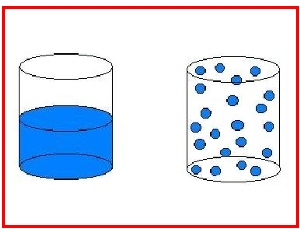
Pore-Space Structure and Fluid Transport in Porous Media |
|||
|
|
|||
|
|
|||
|
|
|||
|
|
|||
|
Multiexponential
relaxation and “pore size” distribution |
|||
|
|
|||
visit "Multiexponential relaxation and local diffusion cells distribution" theory HERE
|
|||
|
|
|||
|
Comparison
between NMR Relaxation time |
|||
|
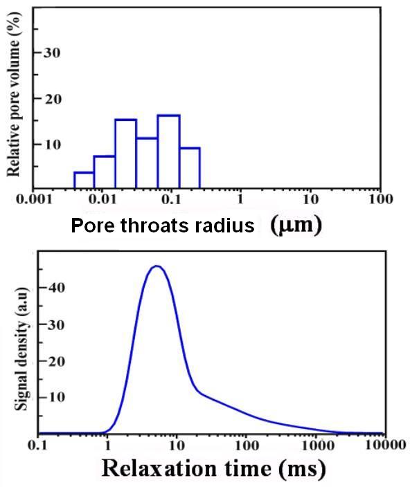
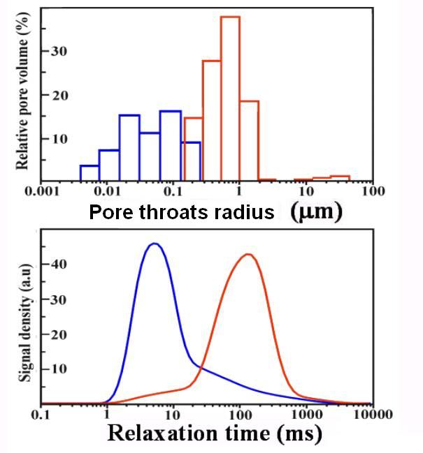
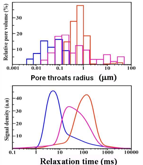
NMR measurements respond to local S/V (or V/S, a length) and are usually calibrated so that distributions of relaxations times correspond to distributions of "pore body" dimensions, whereas Mercury Injection (HgI) measures the pore throat and makes the assumption of a simple geometry for the pore volume. Figures show the distributions of pore throat size by HgI (top) and pore body size by relaxation time (bottom) for a sandstone (yellow), a biocalcarenite (blue), and a marble (green). The agreement between shapes of distributions by both methods and relative positions of the peaks is good, despite the different mineral compositions. With a factor of a little over one order of magnitude one goes from the sandstone to the biocalcarenite, and the marble is in the middle for both methods. A difference is the tail at larger times in the sandstone, which could reflect the presence of low S/V pore spaces that are not connected by other low S/V pores, but rather through smaller pores with smaller throats and therefore underestimated by HgI. Each method gives a portion of information; their combination and integration will give a better insight in our knowledge of the pore space.
|
|||
|
|
|||
|
|
|||
|
|
|||
|
|
|||
|
NMR
Estimation of Permeability |
|||
|
Compact NMR parameters
are needed to estimate single parameter, such as permeability k or
irreducible water saturation Swi,
of oilfield rocks and other porous media. The strategy of
the milestone work of KDSW
(Kenyon, Day, Straley, Willemsen) was to introduce the stretched
exponential time, and to look for the best power laws in the form
kµfBT1C
and proposed kµf4T12. The choice of a form
of “average” time can give emphasis to either the larger or else the
smaller pores, thus giving the possibility of representing different
specific properties of porous media. We used the geometric mean relaxation
time, which emphasizes neither short nor long T1’s
[Magn. Reson. Imaging 14: 751-760 (1996)].
On a suite of about 100 sandstone samples we found that by using the
geometric mean the best estimator is kµf0.94T12.23 , with
an error factor d=1.8.
The isovalue map (on the right) of the error factor δ
as a function of the exponents B and C given to
f
and T1 shows that the surface is rather flat in a wide region where
δ
is not too sensitive to B and C, whereas out of this region the gradients
are very high. This can explain why quite different estimators were
proposed in the literature, with almost the same error factor.
|
|
||
|
In
view of the correlation between f
and the electrical-resistivity formation factor F in sandstones (the classical Archie’s law has the form F=f-m), the same analysis was performed on a subset
of 70 samples, for which formation factors F have been measured. The best
estimator in the form of a power law was
kµF-0.8T1g2.44,
with an error factor d=1.76. |
|
||
|
How to
overcome the Banavar and Schwartz paradox? |
|||
|
|
|||
|
|
|
||
|
The
next step was to get a better insight into the
different
“average"
relaxation times
[Magn. Reson. Imaging 14,
1996, 895-897; J. Appl. Physics 82, 1997, 4197-4204;
Magn. Reson. Imaging
16, 1998, 625-627; Magn. Reson. Imaging 16, 1998, 613-615]. The choice of a form of average time can give emphasis to
longer or shorter times, that
is
to either the larger or else the
smaller pores. Let
us consider the
fractional p-power average T(p)ş<Tp>1/p
|
|||
|
|
|||
|
|
|||
|
|
|||
|
|
|||
|
|
|||
|
|
|||
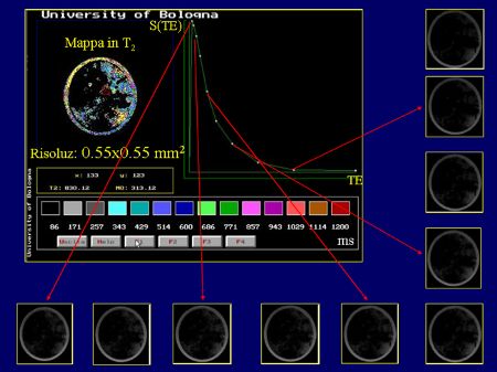
| Relaxation
time maps are generated by means of suitable pulse sequences and
computed by an in-house software written in C++, able to display the maps
and the histograms of relaxation times, with many kinds of different
weightings, for user-defined regions of investigations (ROI’s). S(TE)=S(0)exp(-TE/T2)+k,
where
k is the offset, to get the extrapolated total equilibrium magnetization
S(0) and the T2
value. Then, voxel by voxel,
the signal intensities obtained at different
t values by SR
(Saturation-Recovery) sequences at TE=10 ms were fitted, by introducing the corresponding T2
value of that voxel, to the function S(t)=S(Ą)
[1-k1exp(-t/T1)]exp(-TE/T2)+k2,
where
k1 and k2 are constants, S(Ą)
is the total equilibrium magnetization to be compared with S(0), and T1
is the longitudinal relaxation time to be determined. The assumptions imply the approximation of single-exponential
decay of the transverse and longitudinal components of the 1H
magnetization in each voxel.
|
|||
|
|
|||
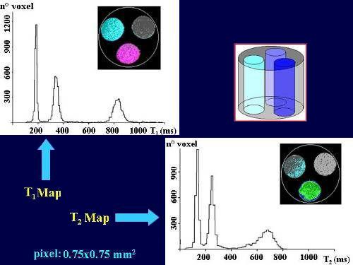
An example is given of the results obtained on a phantom consisting of three tubes containing solutions of EDTA in water at different concentrations. A section of T1 and T2 maps and the corresponding histograms are shown. |
|||
|
|
|||
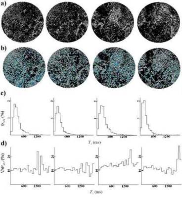
| The figure shows maps obtained from a drained Travertine sample from the Roman Theatre of Aosta. After drainage there remained a saturated porosity of (8.8±0.5)%. The images therefore describe only the water contained in the microporosity or in large pores only weakly coupled with each other, representing about three-fourths of the porosity of the sample. Figures a and b show S(0) and T1 maps, respectively, for four adjacent sections. The signal of each pixel is proportional in S(0) or in T1 maps to the amount of water or to the relaxation time in the corresponding voxel, respectively. The information encoded in the two kinds of maps is different. A voxel with the same amount of water can have a very different T1: a low or high T1 value corresponds to water in high or low S/V regions, respectively. A diffuse microporosity, with regions of lower T1 and higher S/V, is clearly visible in all sections, connected by a network of channels to regions that are partly emptied if they are connected to the external surface of the sample. Many kinds of histograms can be plotted in order to display different characteristics of the pore space. The histograms in Figure c) represent jDT1, which in this case constitutes the microporosity distributed as a function of T1. In this way the area of each column represents the fraction of the total volume of the ROI having that T1 value, and the total area under the histogram represents the microporosity of the selected ROI. Thus, one finds a marked prevalence of T1 corresponding to high values of S/V. Figure d) shows for the same sections the parameter VAPDT1. This parameter is the Volume-Average-Porosity of the voxels having T1 in the selected interval. The distributions start at about 10% for low T1 voxels and tend to increase for higher T1. That means that the pore-volume averages 10% in voxels with quite high specific surface and about twice as much in voxels with larger pores and relatively low specific surface.
|
|||
|
|
|||
|
|
|||